
You’ll discover that the Perform Arguments pane for the IF perform has fields for Logical_test, Value_if_true, and Value_if_false. In our “better than or equal to 18” instance, the logical take a look at is whether or not the quantity within the chosen cell is larger than or equal to 18, the worth if true is “Sure,” and the worth if false is “No.” So we’d enter the next gadgets within the pane’s fields like so:
Logical_test: B2>=18
Value_if_true: “Sure”
Value_if_false: “No”
or simply kind the total components into the goal cell:
=IF(B2>=18,”Sure”,”No”)
This tells Excel that if the worth of cell B2 is larger than or equal to 18, it ought to enter “Sure” within the goal cell. If the worth of cell B2 is lower than 18, it ought to enter “No.”

The IF perform in motion.
Shimon Brathwaite / Foundry
Tip: When utilizing capabilities like this, slightly than coming into the perform repeatedly for every row, you’ll be able to merely click on and drag the tiny sq. on the underside proper of the cell that incorporates the perform. Doing so will autofill every of the rows with the components, and Excel will change your cell references to match. For instance, when the components we utilized in cell C2 that references cell B2 is autofilled into cell C3, it adjustments to reference cell B3 mechanically.

Autofilling a components to subsequent rows within the column.
Shimon Brathwaite / Foundry
Discover extra particulars at Microsoft’s IF perform help web page.
3. The SUMIF and COUNTIF capabilities
SUMIF is a extra superior SUM perform that permits you to add up solely the values in a variety that meet the standards you specify. To make use of this perform, you could specify the vary of cells to use the standards to, the standards for inclusion, and, optionally, the sum vary, which is the vary of cells to complete if that’s completely different from the preliminary vary. The syntax is as follows:
=SUMIF(vary,standards,[sum_range])
Be aware that any standards with textual content or mathematical or logical symbols should be enclosed in double quotes.
Within the gross sales spreadsheet proven under, for instance, suppose you wish to complete up solely the gross sales which might be greater than $100. The factors vary is C2 to C9, and the standards is “better than 100.” Because you’re including up the values in that very same cell vary (C2 to C9), you don’t want to produce a separate sum vary. So your components is:
=SUMIF(C2:C9,”>100″)

Utilizing the SUMIF perform.
Shimon Brathwaite / Foundry
What if as a substitute you wish to discover the entire for all gross sales within the East area solely? To try this you’ll should specify each the standards vary (cells B2 to B9) and the sum vary (cells C2 to C9). That is the components:
=SUMIF(B2:B9,B2,C2:C9)
Be aware that you just don’t should kind out “East” for the standards. You may merely kind B2 or click on the cell B2 to have Excel seek for the textual content it incorporates.

Utilizing SUMIF with each a standards vary and a sum vary.
Shimon Brathwaite / Foundry
There’s a comparable perform known as COUNTIF that permits you to create a depend of values that meet specified standards. The syntax is as follows:
=COUNTIF(vary,standards)
So to depend the entire variety of gross sales within the West area, for example, you provide the vary of cells to use the standards to (B2 to B9), adopted by the standards (“West” or cell B3). The components is:
=COUNTIF(B2:B9,B3)

The COUNTIF perform can immediately depend up gadgets that meet your standards.
Shimon Brathwaite / Foundry
What if you wish to apply a number of standards to your knowledge, similar to calculating complete gross sales for books within the East area, or counting the variety of gross sales over $100 within the West area? Excel can try this too, by way of capabilities known as SUMIFS and COUNTIFS. These capabilities use extra complicated syntax than SUMIF and COUNTIF. For extra particulars, use circumstances, and finest practices for all 4 of those capabilities, see Microsoft’s SUMIF, SUMIFS, COUNTIF, and COUNTIFS help pages.
4. The CONCAT perform
This perform is beneficial for piecing collectively textual content from completely different cells into one full string. As an example, possibly you might have a worksheet with completely different columns for folks’s first and final names, however you wish to put first and final names collectively. Different widespread use circumstances are finishing an tackle, reference quantity, file path, or URL. The syntax is as follows:
=CONCAT(text1,text2,text3,…)
On this instance we’ll use CONCAT to mix a listing of first names and final names right into a full title with an area in between. To take action we merely place the cursor in cell C2, kind =CON and choose CONCAT from the checklist of choices that seems. Subsequent, choose the cell that incorporates the primary title (A2) and add a comma, a clean house surrounded by citation marks, and one other comma. Then add the final title by deciding on the adjoining cell (B2) and hit Enter. Right here’s the total components:
=CONCAT(A2,” “,B2)
Subsequent, click on and drag the underside proper of cell C2 to autofill the components in all the opposite rows.

The CONCAT perform mixed the values from column A with these from column B.
Shimon Brathwaite / Foundry
For extra particulars and examples, see Microsoft’s CONCAT perform help web page.
5. The VLOOKUP perform
This is among the mostly used capabilities in Excel and a priceless knowledge evaluation software. VLOOKUP permits you to lookup a worth in a desk and return info from different columns associated to that worth. It’s very helpful for combining knowledge from completely different lists or evaluating two lists to seek out matching gadgets. To make use of this perform, you should present three to 4 items of knowledge:
- The worth you wish to search for. This is named the lookup worth.
- The vary of cells to look in. This is named the desk array.
- The column that incorporates the data you wish to return, known as the column index quantity.
- Optionally, the kind of lookup you wish to carry out: TRUE or FALSE. This is named the vary lookup. FALSE means you need a precise match for the lookup worth, whereas selecting TRUE returns the most effective approximate match. In the event you don’t specify a variety lookup, VLOOKUP defaults to TRUE.
The syntax is as follows:
=VLOOKUP(lookup_value,table_array,column_index_number,[range_lookup])
The lookup worth should be within the first column of cells you specify within the desk array. The leftmost column within the desk array has a column index variety of 1, with subsequent columns numbered 2, 3, and so forth.
On this instance, we’ll lookup what area our workers work in. To take action, we first must specify the worth that we’re going to seek for: the worker title Mike (cell A2). Subsequent, we have to spotlight all the cell vary (desk array) that we wish to look in: cells F2:G8.
Then we specify which column holds the data that we wish. Fairly than selecting the column itself, we depend from left to proper throughout the desk array. Because the column that incorporates the area is the second from the left, kind in 2.
Lastly, we enter the TRUE (finest approximate match) or FALSE (actual match) possibility. TRUE is usually solely used with numbers or once you aren’t certain if the worth you need is within the desk. Since we all know the worth we wish is within the desk, we’ll decide FALSE. Typically, FALSE is the higher possibility, because it returns extra correct outcomes.
That is the total components:
=VLOOKUP(A2,F2:G8,2,FALSE)

Use VLOOKUP to seek out values linked to different values in massive knowledge units.
Shimon Brathwaite / Foundry
That is an oversimplified instance utilizing a small knowledge set, however when you should search via a spreadsheet with 1000’s (or tens of 1000’s) of cells, VLOOKUP is a large time-saver and reduces the potential for errors. For extra particulars and examples, see Microsoft’s VLOOKUP perform help web page.
Utilizing Copilot to create Excel formulation
Remembering all these completely different formulation and capabilities might be tough, so one other good strategy for many who have entry to Copilot in Excel (see particulars on the prime of this story) is to make use of the AI software to dynamically create formulation that meet your wants. Utilizing Copilot, you’ll be able to describe what you need the components to do and have the AI generate the syntax for you. On this part we’ll display with two pattern knowledge units.
To entry Copilot, click on the Copilot icon in your ribbon toolbar or on the backside proper of your display screen.
To invoke Copilot, click on its icon, which you may discover within the ribbon toolbar up prime or floating on the backside proper of your Excel window.
Shimon Brathwaite / Foundry
The Copilot sidebar opens alongside the best aspect of your spreadsheet. Kind in a immediate describing the components you need created — on this instance, a easy components that provides up all of the gross sales values within the knowledge set. Remember to instruct Copilot the place to put the components:
Create a components in B7 that sums the entire gross sales
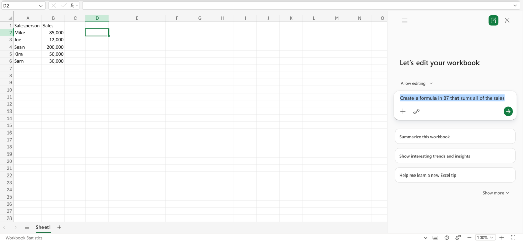
Describe the components you need Copilot to create.
Shimon Brathwaite / Foundry
Click on the submit arrow within the chat window, and Copilot will create and insert the components to provide the end result you need.
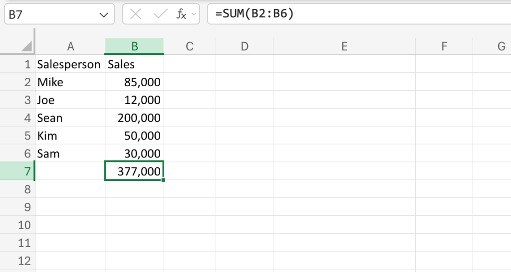
Copilot has inserted the proper Excel components for the sum operation, with the end result showing in cell B7.
Shimon Brathwaite / Foundry
That was a easy one. Now strive a extra superior instance working from a extra complicated knowledge set, as proven within the screenshot under.
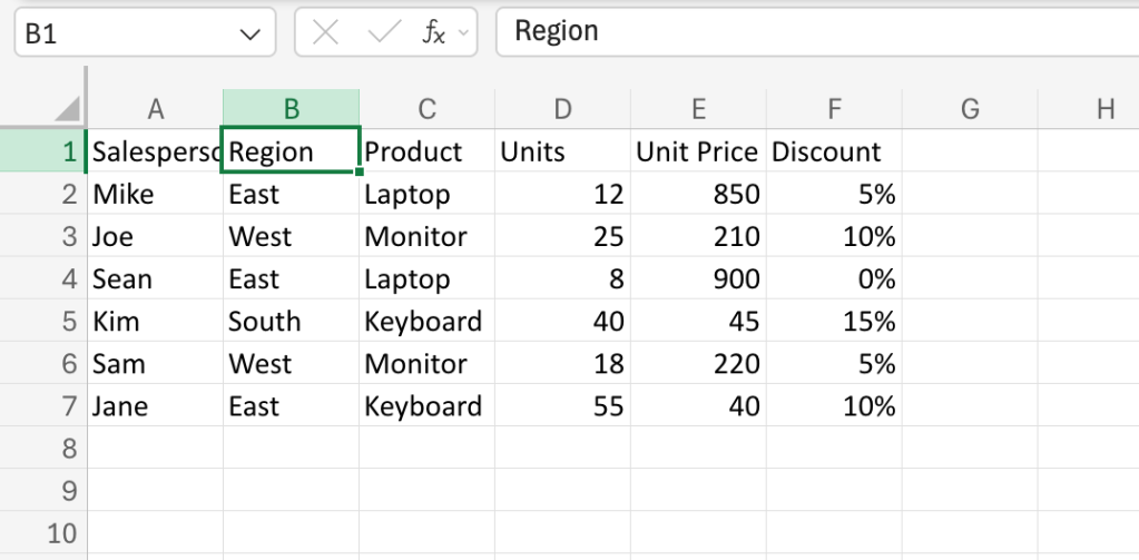
A extra complicated knowledge set for our second instance.
Shimon Brathwaite / Foundry
Strive the next immediate:
Create a components in G2 that calculates complete income per unit whereas accounting for the low cost on every buy. Then fill the components down for all rows and create a abstract desk exhibiting complete income by Area.
Click on the submit arrow, and it ought to create one thing like this:
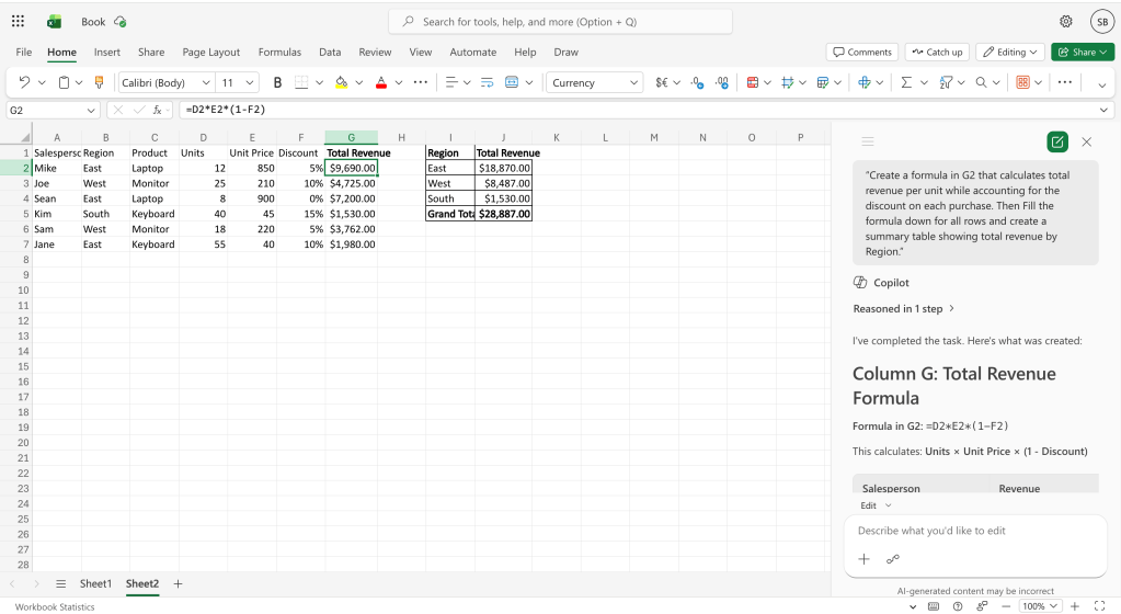
Copilot creates the requested components and fills within the outcomes.
Shimon Brathwaite / Foundry
(There’s much more you’ll be able to have Copilot can do in Excel in addition to creating formulation. See our story “11 cool issues Copilot can do in Excel.”)
Tip: It’s not required, however it may be useful to format your spreadsheet as a desk when working with Copilot. This helps outline extra clearly the precise cells for Copilot to make use of when it creates formulation or takes different actions in your knowledge.
You’re simply getting began
On this story you’ve seen how highly effective formulation and capabilities might be in Excel — and we’ve solely the scratched the floor of what they’ll do. When you get snug utilizing them, you’ll be able to discover a number of the myriad prebuilt capabilities Excel affords and discover ways to construct extra complicated formulation (together with nesting capabilities). That’s all past the scope of this text, however an important place to begin is Microsoft’s “Overview of formulation in Excel” help web page, which incorporates hyperlinks to a number of useful tutorials.
For individuals who have entry to it in Excel, experimenting with Copilot is one other nice approach to study. You may evaluation the steps it took and the formulation it created to get a greater understanding of how formulation work and what they’re able to.
This story was initially printed in Could 2023 and up to date in June 2026.